Parsing the PLoS Corpus dump (tens of thousands or hundreds of thousands!) + SMOG

PLoS Ginormo Corpus

During #opencon a few weeks back the PLoS people announced that the entire corpus was available to download as one giant tar.gz .

The entire corpus of PLOS publications is available as a 3.9gB file here: https://t.co/SNaLt0vjWk #allofplos #opencon
— Brian Nosek (@BrianNosek) November 13, 2016

There was programmatic API access before see this R implementation by ropensci to do it piecemeal, but I’m not sure how much people actually took advantage of it previously.

I thought I’d take a look at it, thinking (foolishly) that it would be a quick and easy thing to parse out the pieces of text I was interested in.

library(readr)
library(tokenizers)
library(dplyr)
library(tidytext)
library(ggplot2)
library(lubridate)
library(tidyr)
library(purrr)
dff=read_csv('journals_abs_sum.csv')
dff$date=ymd(dff$date)
dff=mutate(dff,article=sapply(strsplit(dff$file_name,"_"),function(x) x[[1]][1]))
dffc=filter(dff,simple_abstract==FALSE)
dffc=mutate(dffc,mod_file=paste0('./torrent/abstracts/',dffc$file_name))

JFC parsing XML is a nightmare, and it’s not exactly consistent either

There were actually 2 python phases– for some reason some files I think had been compressed previously (?) and had a few status lines about being uncompressed before the actual xml started - So that needed to be looked for and snipped out to make sure every file is in valid XML format.

After that, I ended up doing the initial parsing with python. xmltodict was the least painful approach I found, and after I massaged out the regions I cared about (abstract to begin with) I wrote it to a new flat file to be read in later by R.

Why was parsing even the abstract complicated?

You may (rightly) be thinking, as I did at first, that once you find part of the dictionary the hard work is done. However- PLoS Abstracts do not have a uniform style format! There is what I’ll call the simple abstract, where it is just one lumped together paragraph, which is easy enough to get out. Then you have “structured” abstracts that have headings like Methods, Results, Conclusion. Then finally, pretty much all plos journals except plos one have a separate “summary” section that is in a perfect world written in human language and not scientific jargon like the abstract, but this is also crammed into the same abstract xml section.

How well did the initial parsing go?

In the first pass I tried to cover the biggest bases, but there are always more edge cases to include. The way I originally counted things for error counting was whether abstracts were “simple” or “structured”. There were 160290 (pretty much all of PLoS One) simple abstracts parsed, and 21825 structured abstracts (all the other plos journals, like biology, genetics, etc.) and 3403 articles where the parser COULDN’T HANDLE and just died. Of the ones that did make it in, they had this distribution:

A tibble: 7 × 2
  journal      n
    <chr>  <int>
  pbio   4541
  pcbi   8494
  pgen  11479
  pmed   1369
  pntd   8207
  pone 157693
  ppat   9661

However, a fair number of the structured abstracts only partially parsed before dying - we can look with the length of the abstract in characters. We can visualize these to get a sense a where the bimodal dip is, and then set a rough cutoff to separate out the articles that clearly failed (there’s also a subset that parse correctly but whose abstract consists essentialy of “we’re not doing an abstract - go to the intro”, which is also not really informative compared to the other texts).

ggplot(aes(x=n_letters,colour=journal,fill=journal),data=dff)+geom_histogram()+theme_minimal()+facet_wrap(~abs_type)+theme(legend.position = c(0.85, 0.7))
ggsave(file='plos_corpus_2016-11-27_corpus_articles_failtail.png',width=7,height=7,dpi=100)
count(dff,journal)

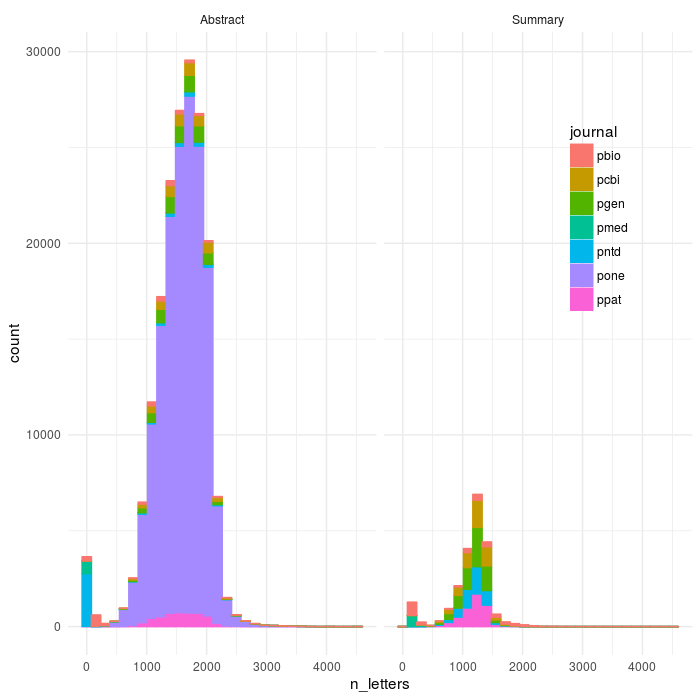
So, what we can see is that as I suspected there are some summaries (and also Abstracts, mostly in pntd, Neglected Tropical Diseases) whose abstract formats is even yet weirder than I accounted for. If we constrain it to be within 500-3000 (you could make this cleaner on either side)

dff2=dff %>%
  group_by(article) %>%
  filter(n_letters>500 & n_letters < 3500) %>%
  ungroup()

df_sep=dffc %>%
  select(article,abs_type,n_letters)%>%#select(journal:abs_type,sentiment:article)%>%
  spread(abs_type,n_letters) %>%
  ungroup()

good_ids=filter(df_sep,Abstract>500 & Abstract <3500 & Summary >500 & Summary < 3500)[,1]

dffc2=dffc %>%
  filter(article %in% good_ids$article) %>%
  mutate(text=sapply(mod_file,function(x) read_file(x)))

#fix stupid article that for ??? reason has time as POSIX instead of YMD like every other sane one
dffc2$date[20097:20098]=ymd(c('2015-11-03','2015-11-03'))

ggplot(aes(x=n_letters,colour=journal,fill=journal),data=dff2)+geom_histogram()+theme_minimal()+facet_wrap(~abs_type)+theme(legend.position = c(0.85, 0.7))
ggsave(file='plos_corpus_2016-11-27_corpus_articles_clean.png',width=7,height=7,dpi=100)
count(dff2,journal)

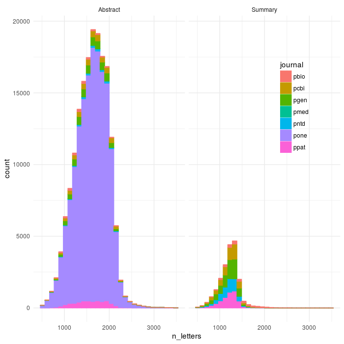
OK, so plos medicine did REALLY bad - I had seen that, they have summaries come before abstracts and I think that breaks everything (I have coded a very dumb parser). Plos Clinical Trials didn’t make it through the parser at all - also need to look into that one more.

Still, it’s a start, yeah?

# A tibble: 7 × 2
  journal      n
    <chr>  <int>
  pbio   2789
  pcbi   8472
  pgen  11451
  pmed     25
  pntd   5435
  pone 157482
  ppat   9646

df_sep=dffc %>%
  select(article,abs_type,n_letters)%>%#select(journal:abs_type,sentiment:article)%>%
  spread(abs_type,n_letters) %>%
  ungroup()

good_ids=filter(df_sep,Abstract>500 & Abstract <3500 & Summary >500 & Summary < 3500)[,1]

df_sep=dffc %>%
  filter(article %in% good_ids$article)

Number of Authors increasing

dffc2=dffc %>%
  filter(article %in% good_ids$article) %>%
  mutate(text=sapply(mod_file,function(x) read_file(x)))

#fix stupid article that for ??? reason has time as POSIX instead of YMD like every other sane one
dffc2$date[20097:20098]=ymd(c('2015-11-03','2015-11-03'))

ggplot(aes(x=date,y=num_authors),data=dffc2)+geom_point()+theme_minimal()+facet_grid(journal~.,scales='free_y')+
  labs(x= "Publication Date",
       y= "Number of Authors (peep those PLoS Genetics numbers)",
       title = "Average number of co-authors of publications in the plos world is rising")

ggsave(file='plos_corpus_2016-11-27_date_authors_scatter.png',width=7,height=7,dpi=100)

dft=select(dffc2,article,abs_type,text)
#follow nesting via silge ~blog~ example
dftn=dft %>% 
  group_by(article,abs_type) %>%
  nest() %>%
  mutate(tidied = map(data, unnest_tokens, 'sentence', 'text', token = 'sentences'))

dftn = dftn %>%
  unnest(tidied)

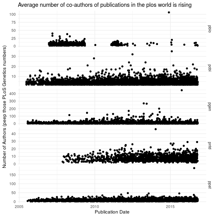
Authors are increasingly numerous - check out the y axis on the plos Genetics!

Amazing tidy and tidytext skillz + tricks c/o Julia Silge

I had been working parsing the XML and improving the basic numbers for a few days, when to my immense benefit Julia Silge posted an analysis on SMOG (wordiness) over Thanksgiving break.

One of the basic analyses I had in mind was comparing these abstract and author summary regions in a few different ways. The first was just sentiment, but although I hadn’t heard of SMOG before it seemed perfectly suited to what I had in mind; serendipity at its best.

I definitely recommend checking out her post, I hadn’t come across nesting via tidyr and it’s quite useful, as is the ggstance package.

The following snippit is the really time-consuming bit of code to algorithmically count syllables (the other option being to use say a dictionary). The code comes from Tyler Kendall at here. It took about an hour with the subset of ~50k cleaned texts with paired abstract and summary sections. There’s another 160k or so (almost exclusive PLOS One, as I’ve mentioned) that I haven’t really had a chance to touch yet, but will obviously take quite awhile longer to work through.

dftn= dftn %>% 
  unnest_tokens(word, sentence, drop = FALSE) %>%
  rowwise() %>%
  mutate(n_syllables = english_syllable_count(word)) %>%
  ungroup()


df_join=inner_join(dftn,select(dffc2,journal,num_authors,sentiment,date,n_letters,article,abs_type))

Sentiment in Abstract vs Summary across journals

When I was extracting the abstract and summary sections from the articles, I went ahead and calculated sentiment in python using one of the tools in that ecosystem , the vader package from nltk. vader is based off short texts and blogs, but seems to do well for non-social media as well. It is a full sentence parser, and uses information about modifiers of speech.

library(purrr)
library(ggstance)
library(ggthemes)
library(forcats)

results <- left_join(dftn %>%
                         group_by(article,abs_type) %>%
                         summarise(n_sentences = n_distinct(sentence)),
                     dftn %>% 
                         group_by(article,abs_type) %>% 
                         filter(n_syllables >= 3) %>% 
                         summarise(n_polysyllables = n())) %>%
    mutate(SMOG = 1.0430 * sqrt(30 * n_polysyllables/n_sentences) + 3.1291)

results2=inner_join(results,select(dffc2,journal,num_authors,sentiment,date,n_letters,article,abs_type))

ggplot(aes(x=abs_type,y=sentiment),data=results2)+
  geom_boxplot()+ 
  theme_minimal()+
  facet_wrap(~journal)+
  labs(x='Abstract Section',y='Vader Sentiment',
       title="Sad Trombone- Seems like journal but not abs./sum. sent. var.",
       subtitle="todo-check if the zinger last sentence is important?")

ggsave(file='plos_corpus_2016-11-27_sentiment_journal.png',width=7,height=7,dpi=100)

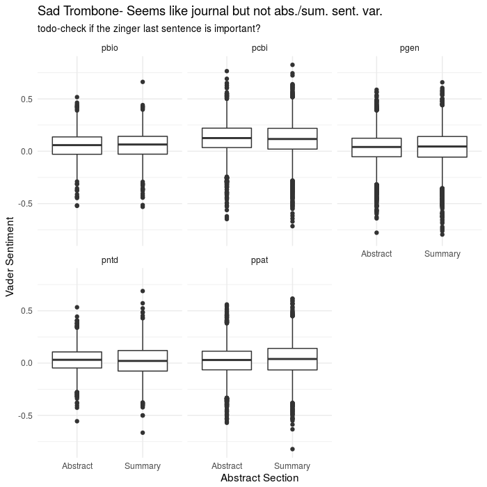
That analysis didn’t work out so great

So, obviously when doing ~data science~ or whatever you want to call mucking about like this, things won’t always pan out. I had originally anticipated finding some correlation between sentiment and abstract type, especially based on this amusing/depressing paper on the use of positive and negative words in pubmed abstracts. The BMJ, British Medical Journal, if you didn’t know, has a tradition of publishing some more “off the beaten path” papers for their christmas edition, that are still rigorous enough. They looked at all pubmed abstracts going back to the 70s, but had a screen of ~25 positive and negative words and were concerned just with the change in frequency (spoiler: people have gotten more bombastic in recent years and everything is AMAZING and CRITICAL now).

However, if you’ve written a scientific paper, or really anything, the emphasis and point of a well-written paragraph will usually come in the last sentence. Having worked my way through several confusing papers, this typically manifests as several sentences of “this worked, this didn’t”, and then at the end, stepping back and saying something sweeping like “These results indicate that an important aspect of x is the role played by y”, perhaps in even more glowing terms. So what does the sentiment look like if we just look at the last sentence in isolation, which should be “peak optimist” in terms of writing?

TODO

PLoS syllables and SMOG ranking

These are minor variations on Julia Silge’s blog post, so I won’t delve into the background too much. I should note, however, that the SMOG wikipedia article notes that it was normalized on 30 sentence texts; these abstracts are a fair bit shorter. I guess what I’m trying to say is that take it with a grain of salt that is also maybe a bit on fire.

ggplot(aes(n_syllables, fill = journal, color = journal),data=df_join) +
  facet_wrap(~abs_type) +
  geom_density(alpha = 0.0, size = 1.1, adjust = 9) +
  theme_minimal() +
  theme(legend.title=element_blank()) +
  theme(legend.position = c(0.8, 0.7)) +
  labs(x = "Number of syllables per word",
       y = "Density",
       title = "Comparing syllables per word across journals abstracts and summaries",
       subtitle = "Not much difference in article and summary syllable dist. aggregates")

ggsave(file='plos_corpus_2016-11-27_syllables.png',width=7,height=7,dpi=100)

ggplot(aes(x=journal,y=SMOG),data=results2) +
  geom_boxplot(aes(colour=abs_type)) +
  theme(legend.title=element_blank()) +
  theme_minimal()+
  labs(x='Journal',y='SMOG (Wordiness)',
       title="Author summary somewhat less jargon filled than full abstract")
ggsave(file='plos_corpus_2016-11-27_smog.png',width=7,height=7,dpi=100)

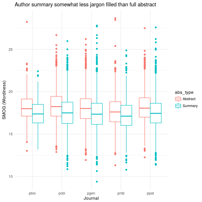
This one actually turned out pretty well, I thought. Aside from the whole not exactly being valid because the texts are too short. It at least goes with the expectation that the summary would be more readable than the true abstract.

Looking forward, and requisite caveat

So, what did we learn? Well, as a first pass there’s quite a trove of stuff to be had in the corpus, it’s quite a large dataset. However, there is also a fair bit of complexity in terms of parsing the xml structure, given that there are so many exceptions. The way I’ve taken to started working with my code is to start building out short functions that parse out the sections that I’m interested in, such as the author listing, etc.

Most of the analyses presented thus far were based on the subset of texts that have both an abstract and an author summary - pretty much everything that’s not plos One. On the other hand, that means I’ve also excluded 160k abstracts just because I wanted to focus on a subset of 22k articles in the panople of the PLoS “premium” journals of first (it was also smaller by nature).

I haven’t really looked into it at all yet, but parsing the body of the paper would be similar in nature to structured abstract, except you need to look for sections that are called “introduction” “methods”, etc. The exceptions will be that not all will follow that order, or be called those. So maybe take everything except the headings that correspond to figure and table sections? The XML in the body is a bit of a mess, really.

Anyway, it’s super early days so some parts of the parser worked better than others, as parts of the journals meshed better or worse with my terrible parser. PLoS medicine for instance, did awful (only 25 main it into the clean dataset). PloS biology also had tons of time gaps, probably more due to failures in parsing than missing a summary. Something to investigate more when I get a chance, anyway. The other journals (like Genetics, Pathogens, Computational Biology, etc.), seemed to have a more regular style that conformed to my initial logic.