Incorporation of Hedonometer lexicon to Tidytext
The paper by Dodds et al. in 2011 introduced the concept of the Hedonometer, which measures one specific gradient of emotion, happiness or its inverse sadness - to the Twitter platform.
They mentioned that the day of the election was the third saddest day on Twitter (the others being the Pulse and Dallas shootings).
Yesterday was the third saddest day in the history of Twitterhttps://t.co/bQDYojAVF2 pic.twitter.com/MMPGRWh4j6
— hedonometer (@hedonometer) November 10, 2016
This past month has been somewhat rough, and the election outcome was quite a shock and dismay to me. As a small project of introspection and self-care, I wanted to see how the sentiment in my Twitter time-line has changed in and around the election using this metric.
At first I thought I would be limited to the last 3200 tweets (the API limit for user timelines), but reading Silge and Robinson’s book (see the next section), you can get your full twitter archive by going to your twitter setting and clicking on archive and waiting for the email.
Twitter Usage (Frequency)
The first few graphs I want to show are some simple ones I have (or haven’t) used Twitter over the years
library(twitteR)
library(tidytext)
library(ggplot2)
library(wordcloud)
library(dplyr)
library(stringr)
library(tm)
library(readr)
library(lubridate)
library(cowplot)

load('twitter-secrets.Rdata')
setup_twitter_oauth(cons_key,cons_sec, acc_tok, acc_sec)

# will leave in for posterity - can use to get other user timelines -
#mytweets=userTimeline('tek_keller',n=3200,includeRts=T)
#tw_df<-twListToDF(mytweets)
#write.csv(tw_df,file='tek_timeline11-12-16.csv',row.names=F)
tw_df=read_csv('tek_tweets_all6k.csv')

confname='TEK'

tw_df$timestamp=with_tz(ymd_hms(tw_df$timestamp),"EST")

ggplot(tw_df, aes(x = timestamp)) + geom_histogram(position = "identity")
ggsave(file='tek_hist_alltweets.png',width=7,height=7,dpi=100)

tw_df2=filter(tw_df,timestamp>= "2016-01-01" & timestamp <= "2016-12-31")

ggplot(tw_df2, aes(x = timestamp)) + geom_histogram(position = "identity")
ggsave(file='tek_hist_just2016.png',width=7,height=7,dpi=100)
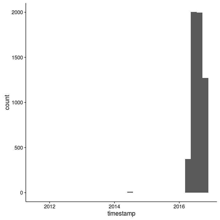
The histogram of tweets through time is pretty hilarious, but also reflective of about how I have used social media in recent years (I haven’t, generally; my Facebook is similarly spartan). However, when I finished up my last postdoc in December of last year I realized I needed some way of staying connected to people and science in the larger world while I was figuring out what to do next and I wasn’t physically connected to a university. Hence you can see me dusting off ye olde Twitter account in the spring of 2016.
In fact, I made a total of 15 tweets in the prior 4 years so it’s simpler to just cut that time out and focus on my more recent “shit-posting”, I mean science-posting!
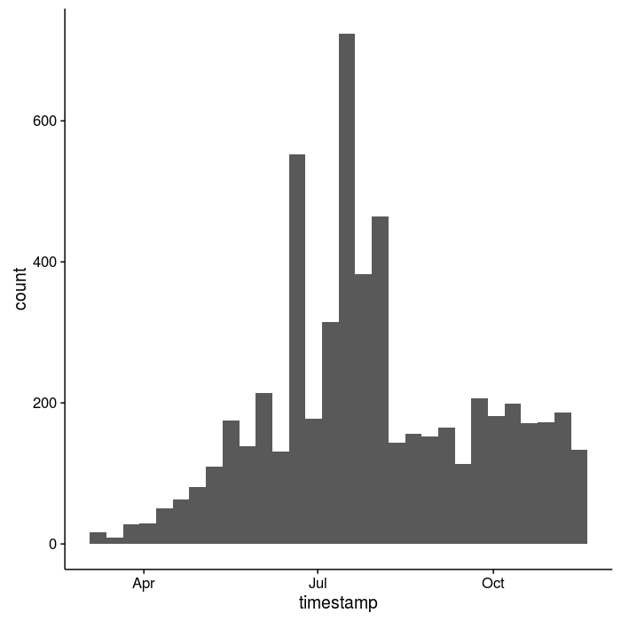
The summer months were heavily elevated (conferences and my attempts at #scicomm), but otherwise I seem to have a somewhat regular state of tweeting.
Regex Monstrosties and unnesting tokens
The beginning of this code comes from Julia and Dave’s wonderful new book TidyText Mining with R. Specifically, the section on Twitter. Twitter has certain weird characteristics that make the default unnesting unpalatable-namely stripping the # and @ from words, which are quite important features for downstream analyses! Therefore, we have go to some horrific regex lengths to work around these default assumptions in the unnesting framework.
Part of my TODO is to figure out how this REGEX (either the first or second part) is working.
library(tidytext)
library(stringr)
reg <- "([^A-Za-z_\\d#@']|'(?![A-Za-z_\\d#@]))"
tidy_tweets <- tw_df2 %>%
mutate(text = str_replace_all(text, "https://t.co/[A-Za-z\\d]+|https://[A-Za-z\\d]+|http://[A-Za-z\\d]+|&|<|>|RT", "")) %>%
unnest_tokens(word, text, token = "regex", pattern = reg) %>%
filter(!word %in% stop_words$word,
str_detect(word, "[a-z]"))
tidy_tweets2 = tidy_tweets %>% filter(!str_detect(word, "@"))
frequency <- tidy_tweets2 %>%
count(word, sort = TRUE) %>%
mutate(total = n(), freq=n/total)
filename='tek_twitter_words.png'
png(filename, width=12, height=8, units="in", res=300)
wordcloud(frequency$word,frequency$n,max.words = 100,colors=brewer.pal(8,'Dark2'))
dev.off()
frequency
Requisite wordcloud monstrosity
Here in the ball of words below, you’ll see some of my interests over the last year. One important, actually HUGE caveat is that I haven’t separated out retweets from my own tweets in this analysis. In part that’s because I’m not a very vocal tweeter still, I tend towards finding interesting accounts and retweeting stuff I find interesting. Definitely something to look back on the reduced, smaller dataset of just my own tweets, few as they are.
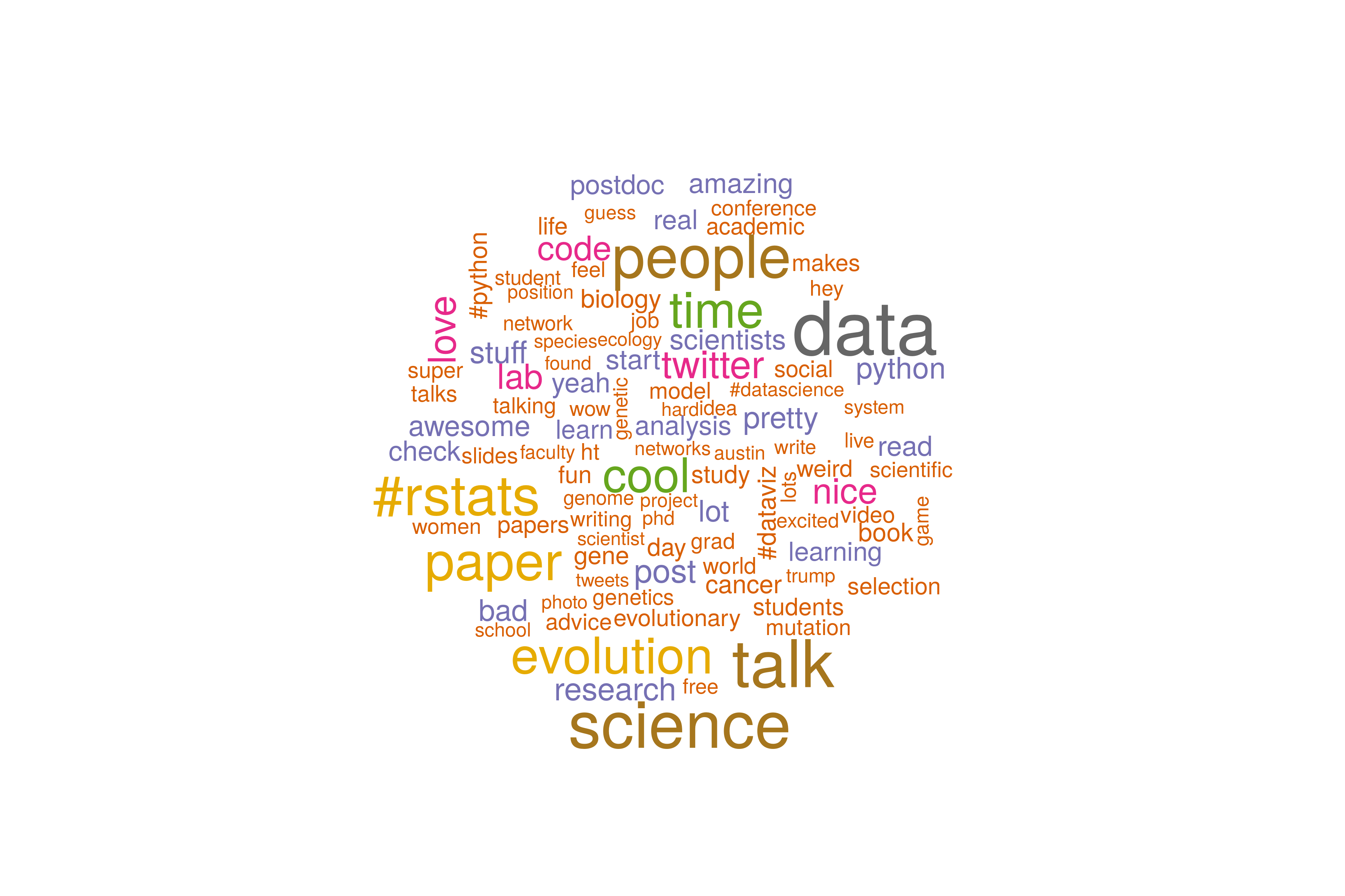
The big hashtags #Evol2016 and #TGCA2016 refer to the two big biology conferences that I went to this year (actually I deleted these because they were too big and throwing things off). I met some great people, and saw a bunch of old friends. Evolution was especially great, with it being in Austin and all. The adjusted wordcloud now has seasonally appropriate fall coloring, as an unintentional bonus.
The parsing and regex (notably the str_replace_all) didn’t quite work as planned, there’s still some https and and htt hanging around. Probably the thing to do is a bind_row and then an filter with the extra stop words appended.
Tracking emotion with the Hedonometer
So, now to the actual analysis with the Hedonometer - basically this is just taking in the data from the Mechanical Turk assessment of words (Table S1 in the paper), though I did normalize the values from the 1-9 scale they use to -1 to 1 which is a bit easier to wrap your head around (after the grading has been done; initial scale makes total sense). You can a more fully fleshed-out python implementation at this nicely named sentimenticon.
library(tidytext)
library(readr)
hdf=read_tsv('Dodds_etal2011_Hedonometer_lexicon10k.txt',skip=3)
hdf=mutate(hdf,happiness_norm=(((((happiness_average-1)) / 8 * 2) -1)))
hdf2=filter(hdf,!(happiness_average>=4 & happiness_average <=6) )


hed_sent = tidy_tweets2 %>%
  inner_join(hdf2) %>%
  group_by(tweet_id) %>%
  summarise(sum_happy=sum(happiness_norm)) %>%
  inner_join(tidy_tweets2[,c(1,4)]) #merge on id and timestamp


conf_sent <- tidy_tw %>%
 inner_join(bing) %>%
 count(id, sentiment) %>%
 spread(sentiment, n, fill = 0) %>%
 mutate(sentiment = positive - negative) %>%
 inner_join(tw_df[,c(5,8)]) #join on id and created

library(cowplot)
library(scales)
library(lubridate)


#Example could include label, but don't have time to figure out what is driving
#inflection points of moods during these other conferences

ggplot(hed_sent, aes(timestamp, sum_happy)) +
 geom_smooth() + xlab("tweet time") + ylab("tweet sentiment")+
 scale_x_datetime(breaks = date_breaks("month")) + background_grid(major = "xy", minor = "none") +
 theme(axis.text.x=element_text(angle=315,vjust=.6))+
  #geom_text(data=df_labels,aes(x=times,y=y,label=labels),size=4)+
  ggtitle(paste("Hedonometer of TEK tweets (includes retweets) over past year"))
 #coord_cartesian(ylim=c(-.5,1.2)) #+geom_text(data=df_labels,aes(x=times,y=y,label=labels),size=4)

filename<-paste0("tek_hedonometer_2016.png")
ggsave(file=filename,width=7,height=7,dpi=100)
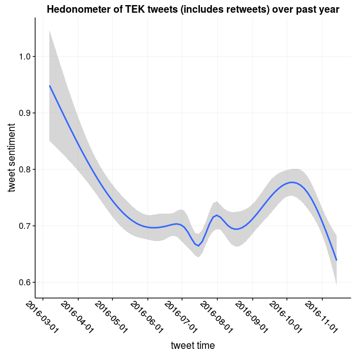
As you can see, there has been a gradual, slight decline in positivity at the beginning of the year towards some kind of middle ground of ~0.7 around May with some bumps (conferences) in the summer, with an increase in September and then a sharper decrease in November. I won’t overanalyze myself, but that fits with about how my year has gone. I’ve been trying to figure out where I want to go after I finished my postdoc last December, and have yet to have a permanent full time job lined up. For awhile I thought I’d go into ~data science~ but that seems like that might not be the best fit for me (I miss biology too much), so in September I was fortunate enough to have the opportunity to come back up to Atlanta to work with my advisor Dr. Yi to do some machine learning on some biological datasets (hopefully an upcoming post; I need to get back to blogging). That matches with the uptick in mood, it was really nice to be back in an office environment after applying for a bunch of jobs without luck (I suppose I was too restrictive in trying to stay near parents in Tampa).
The Election Event
In any case, the original point and question for the post was: how and to what extent did the election affect my mood? The prior plot suggests that there wasn’t a huge change, and any change was part of a larger downturn in emotion over the last month.
df_labels<-data.frame(times=strptime("2016-11-08 6:00:00","%Y-%m-%d %H:%M:%S"),
                      labels=c("The Event"),
                      y=c(1.2))
hed_sent2=filter(hed_sent,timestamp>="2016-11-01")
ggplot(hed_sent2, aes(timestamp, sum_happy)) +
 geom_smooth() + xlab("tweet time") + ylab("tweet sentiment")+
 scale_x_datetime(breaks = date_breaks("day")) + background_grid(major = "xy", minor = "none") +
 theme(axis.text.x=element_text(angle=315,vjust=.6))+
  geom_text(data=df_labels,aes(x=times,y=y,label=labels),size=4)+
  ggtitle(paste("Hedonometer of TEK tweets (includes retweets) over month"))
filename<-paste0("tek_hedonometer_election.png")
ggsave(file=filename,width=7,height=7,dpi=100)

 #coord_cartesian(ylim=c(-.5,1.2)) #+geom_text(data=df_labels,aes(x=times,y=y,label=labels),size=4)
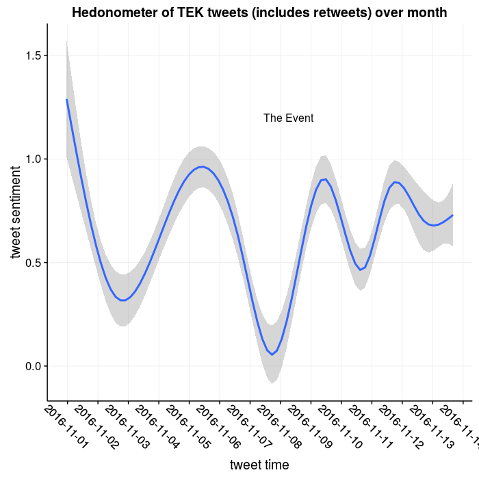
No real surprise, I guess. There was indeed a big dip on election day, though its somewhat evened out over the last few days. I’m still processing what this election means. In some ways, as a white dude I can just put my head down and soldier on. However, I have a lot of friends who are vastly more negatively affected than this election than I am, and it weighs on my mind.
My plan is to donate monetarily to some organizations once I’m (hopefully) hired to a permanent position somewhere in the coming months, but in the meantime I will probably do some volunteer work to ease the existential angst I’m feeling. It’s easy to say something and then forgot about it once the initial shock and horror fades away (such as this election), my hope is that in writing it I won’t forget my obligations.
Time to get out of the doldrums, in any case.